|
|
|
 |
|
|
共分散構造分析ソフトウェア
Amos 4
(Windows95/98/NT4.0/2000版) |
|
Amos のグラフィック・モデル機能
例 4: Conventional Linear Regression
入力データ
Warren, White and Fuller (1974) studied 98 managers of farm cooperatives. Four of the measurements obtained from each manager were
performance
A 24-item test of performance related to "planning, organization, controlling, coordinating and directing."
knowledge
A 26-item test of knowledge of "economic phases of management directed toward profit-making ... and product knowledge."
value
A 30-item test of "tendency to rationally evaluate means to an economic end."
satisfaction
A 11-item test of "gratification obtained ... from performing the managerial role."
The sample variances and covariances are:
| |
performance |
knowledge |
value |
satisfaction |
|
----------- |
----------- |
----------- |
----------- |
| performance |
.0209 |
|
|
|
| knowledge |
.0177 |
.0520 |
|
|
| value |
.0254 |
.0280 |
.1212 |
|
| satisfaction |
.0046 |
.0044 |
-.0063 |
.0901 |
In the linear regression model, the performance scores are predicted by the knowledge, value and satisfaction scores.
The regression model can be specified in equation form in Amos Text ...
$Structure
performance = knowledge + value + satisfaction + error (1)
... or as a path diagram in Amos Graphics
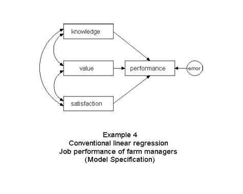
By convention, observed variables are displayed in rectangles, latent variables (or variance components) in circles or ellipses.
Example 5: Regression with errors in variables
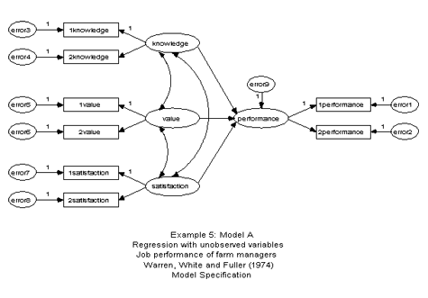
These data are from the same study as the previous example, except that the sample moments are for split-half tests constructed by randomly dividing up the items of each test. With the covariance information of the split-half tests, measurement errors and the disattenuated prediction model can be estimated simultaneously.
Input data
! Managerial Role Performance of Farm Managers
! Sample means from Warren, White, and Fuller (1974).
! Sample covariance matrix from Joreskog and Sorbom (1984).
$Sample size = 98
$Input variables
1performance ! 12-item subtest of Role Performance
2performance ! 12-item subtest of Role Performance
1knowledge ! 13-item subtest of Knowledge
2knowledge ! 13-item subtest of Knowledge
1value ! 15-item subtest of Value Orientation
2value ! 15-item subtest of Value Orientation
1satisfaction ! 5-item subtest of Role Satisfaction
2satisfaction ! 6-item subtest of Role Satisfaction
past_training ! Degree of formal education
$Covariances
.0271
.0172 .0222
.0219 .0193 .0876
.0164 .0130 .0317 .0568
.0284 .0294 .0383 .0151 .1826
.0217 .0185 .0356 .0230 .0774 .1473
.0083 .0011 -.0001 .0055 -.0087 -.0069 .1137
.0074 .0015 .0035 .0089 -.0007 -.0088 .0722 .1024
.0180 .0194 .0203 .0182 .0563 .0142 -.0056
-.0077 .0946
$Means
0.0646 0.0542 1.4333 1.3259 2.8404 2.9143 2.4514 2.4711
2.1174
Model specification
Example 6: Stability of alienation study
Input data
! Alienation and socioeconomic status.
! Correlations, standard deviation and means
! from Wheaton et al. (1977).
$Inputvariables
anomia67 ! Anomia score in 1967
powles67 ! Powerlessness score in 1967
anomia71 ! Anomia score in 1971
powles71 ! Powerlessness score in 1971
education ! Years of schooling completed in 1966
sei ! Socioeconomic index, measured in 1966
$Samplesize=932
$Correlations
1.00
.66 1.00
.56 .47 1.00
.44 .52 .67 1.00
-.36 -.41 -.35 -.37 1.00
-.30 -.29 -.29 -.28 .54 1.00
$Standard deviations
3.44 3.06 3.54 3.16 3.10 21.22
$Means
13.61 14.76 14.13 14.90 10.90 37.49
Model specification
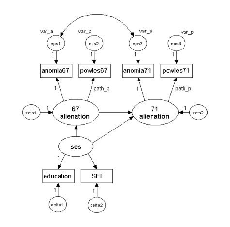
This panel study obtained measurements of the same anomia and powerlessness variables in 1967 and 1971. With Amos, it is easy to specify a time-invariant measurement model. Whenever the same label is used for two (or more) parameters, Amos restricts these parameters to the same value.
Example 7: Perceived attractiveness and academic ability in girls (non-recursive model)
Input data
! Felson and Bohrnstedt (1979)
! study of perceived attractiveness and academic
! ability in teenagers, sixth through eighth grade.
$Input variables
academic ! Perception of academic ability.
athletic ! Perception of athletic ability.
attract ! Perception of physical attractiveness.
GPA ! Grade point average.
height ! Height minus group mean for age and sex.
weight ! Weight with height 'controlled'.
rating ! Strangers' rating of attractiveness.
$Sample size = 209
$Correlations
1.00
.43 1.00
.50 .48 1.00
.49 .22 .32 1.00
.10 -.04 -.03 .18 1.00
.04 .02 -.16 -.10 .34 1.00
.09 .14 .43 .15 -.16 -.27 1.00
$Standard deviations
.16 .07 .49 3.49 2.91 19.32 1.01
$Means
.12 .05 .42 10.34 .00 94.13 2.65
Model specification
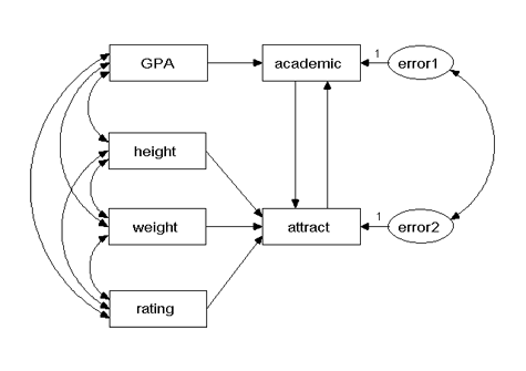
This model allows the ratings of attractiveness and academic performance to simultaneously affect each other.
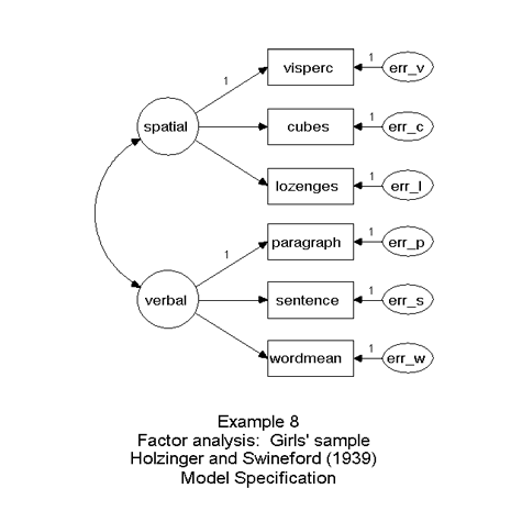
Example 8: Two-factor model of 6 psychological tests
Input data
! Holzinger and Swineford (1939) Grant-White sample.
! Intelligence factor study. Raw data of 73 female
! students from the Grant-White high school, Chicago.
$Input variables
visperc ! Visual perception score
cubes ! Test of spatial visualization
lozenges ! Test of spatial orientation
paragraph ! Paragraph comprehension score
sentence ! Sentence completion score
wordmean ! Word meaning test score
$Sample size = 73
$Raw data
33. 22. 17. 8. 17. 10.
30. 25. 20. 10. 23. 18.
36. 33. 36. 17. 25. 41.
... (67 similar lines omitted about here)
35. 28. 10. 9. 13. 11.
18. 24. 13. 7. 16. 7.
28. 22. 15. 11. 23. 30.
Model specification
Factor models can have unobserved predictors (or factors). These may also be interpreted as variance components.
Example 11: Perceived attractiveness and academic ability (two-group analysis of girls' and boys' samples)
The model has the same general structure for the two groups of respondents, girls and boys. The path coefficients are labeled g1-g6 and b1-b6, respectively, in the girls' and boys' models.
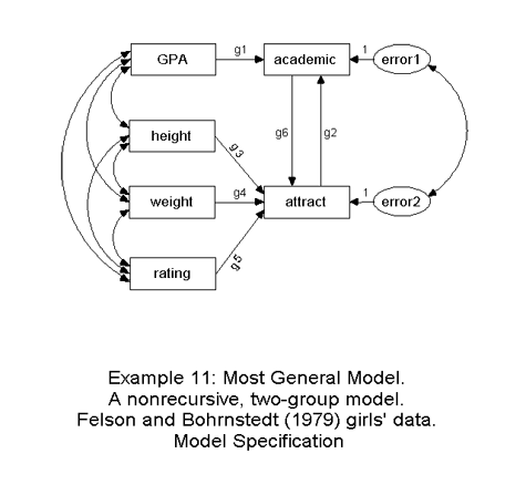
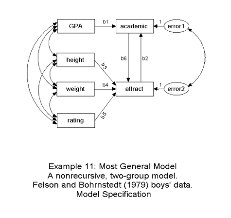
New models can be defined via parameter constraints. While, under Model_A (below), each free parameter may have different values in the two groups, Model_B postulates six of the path coefficients as group-invariant. Both models are specified and analyzed simultaneously. Amos calculates several statistics for evaluating absolute and relative fit of nested models.
$Model = Model_A
$Model = Model_B
b1 = g1
b2 = g2
b3 = g3
b4 = g4
b5 = g5
b6 = g6
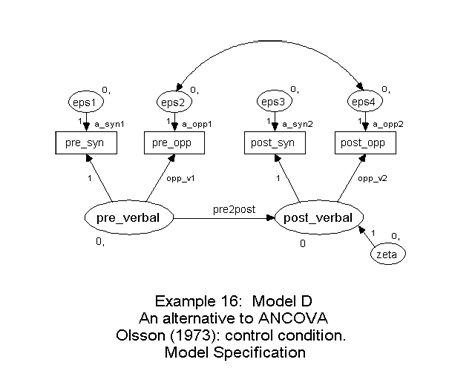
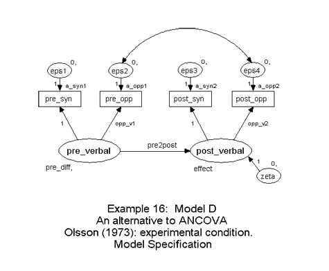
Example 16: Latent variable regression in two groups
Parameters can also be made group-invariant by simply giving them the same label in each group. Additional equality constraints can be imposed by $Model commands, as shown in Example 11.
|
| Amos 4のTopページに戻る |
|
|

