|
|
|
 |
|
|
時系列分析ソフトウェア
RATS |
|
3-5. RATS Basics: Ordinary Least Squares Regressions
The basic instruction for estimating ordinary least squares (and related) regressions is LINREG. The general syntax of LINREG is shown below:
LINREG(options) dependentvariable start end residuals # list of regressors
The items in italics are called parameters. Parameters are generally used for supplying information such as series names and starting and ending dates. The second line, beginning with the "#" symbol, is called a supplementary card. Many instructions use supplementary cards for supplying additional information. For LINREG, you specify the right-hand-side variables on the supplementary card.
Our Example Program
We want to regress food consumption on a constant, retail prices, disposable income, and a time trend, using ordinary least squares. Here's the instruction that does just that:
LINREG FOODCONS # CONSTANT PRRETAIL DISPINC TREND
In this example, FOODCONS is the dependent variable. We've omitted the start and end parameters, so RATS will automatically use all available data for the regression. We've also omitted the residuals parameter, which can be used to save the residuals in a series. We supply the names of our regressors on the supplementary card.
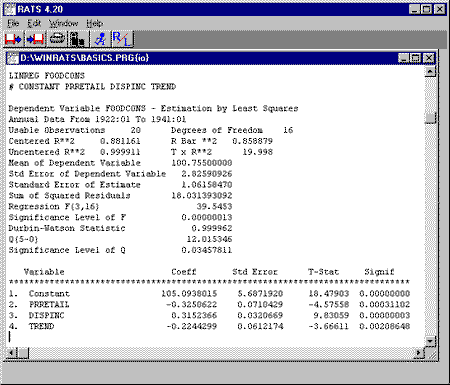
Below is a screen shot showing the above instruction and the resulting output:

As you can see, RATS displays a lot of output, in a very readable format. Most of the statistics displayed here are also stored into special reserved variables, so you can use them in subsequent calculations. For example, the number of degrees of freedom is stored in the variable %NDF and the adjusted R-squared statistic is stored in the variable %RBARSQ.
RATS makes it easy to specify lags in regression models. The following instruction regresses food consumption on a constant, retail prices, and both the contemporaneous (zero lag) and one-period lag of disposable income:
LINREG FOODCONS # CONSTANT PRRETAIL DISPINC{0 1}
Other Examples
Suppose you want to regress long-term interest rates on lags zero (contemporaneous entry) through 24 of short-term interest rates. You could list each lag separately, but it is easier to use the "TO" notation to specify a range of lags. For example:
LINREG LONGRATE # CONSTANT SHORTRATE{0 TO 24}
Like all of the estimation instructions, LINREG offers various options for doing different kinds of estimations, controlling output, defining equations, and more. The examples below demonstrate the ROBUSTERRORS option, which corrects the covariance matrix for heteroscedasticity, and the INSTRUMENTS option, which, when combined with the INSTRUMENTS instruction, does two-stage least squares.
This regresses GNP on a constant and 4 leads and 8 lags of M1, and corrects the covariance matrix for heteroscedasticity:
LINREG(ROBUSTERRORS) GNP 55:1 86:4 # CONSTANT
M1{-4 TO 8}
This computes 2SLS estimates of CONS on GNP and lagged CONS, using the list of instrumental variables defined by the INSTRUMENTS instruction (the $ symbol on the INSTRUMENTS instruction indicates that the instruction continues on the next line):
INSTRUMENTS
CONSTANT MDIFF{0 1} GOVT{0 1} INVEST{1} CONS{1 2} $ GNP{1 2} RATE{1 TO 5}
LINREG(INSTRUMENTS) CONS # CONSTANT GNP CONS{1}
We'll demonstrate some other estimation techniques later on. First, however, we'll look at hypothesis testing and forecasting.
|
|
|
|
| ←RATSのTopページに戻る |
|
|

